rbtl - Data wrangling with tidyr

Lars Schöbitz

Global Health Engineering - ETH Zurich

2022-05-19

Today

Part 1: Data types and vectors
- Live Coding Exercise
Part 2: tidyr - long and wide formats
- Live Coding Exercise
Part 3: dplyr - joining data
- Live Coding Exercise
Homework Assignment 13
Programming Exercise

Learning Objectives

Learners can apply functions from the ~~tidyr~~ (actually dplyr) R Package to join multiple data sets
Learners can apply functions from the tidyr R Package to transform their data from a wide to a long format and vice versa

Part 1: Data types and vectors

Why care about data types?

via GIPHY

Example: survey data

survey_data_small

# A tibble: 22 × 3
     id job      price_glass
  <int> <chr>    <chr>      
1     1 Student  0          
2     2 Retired  0          
3     3 Other    0          
4     4 Employed 10         
5     5 Employed See comment
6     6 Student  05-Oct     
# … with 16 more rows

Oh why won’t you work?!

survey_data_small %>% 
  summarise(mean_price_glass = mean(price_glass))

# A tibble: 1 × 1
  mean_price_glass
             <dbl>
1               NA

Oh why won’t you still work??!!

survey_data_small %>% 
  summarise(mean_price_glass = mean(price_glass, na.rm = TRUE))

# A tibble: 1 × 1
  mean_price_glass
             <dbl>
1               NA

Take a breath and look at your data

glimpse(survey_data_small)

Rows: 22
Columns: 3
$ id          <int> 1, 2, 3, 4, 5, 6, 7, 8, 9, 10, 11, 12, 13, …
$ job         <chr> "Student", "Retired", "Other", "Employed", …
$ price_glass <chr> "0", "0", "0", "10", "See comment", "05-Oct…

Very common data tidying step!

survey_data_small %>% 
  mutate(price_glass_new = case_when(
    price_glass == "5 to 10" ~ "7.5",
    price_glass == "05-Oct" ~ "7.5",
    str_detect(price_glass, pattern = "20") == TRUE ~ "20",
    str_detect(price_glass, pattern = "See comment") == TRUE ~ NA_character_,
    TRUE ~ price_glass
  ))

Very common data tidying step!

# A tibble: 22 × 4
      id job      price_glass_new price_glass                    
   <int> <chr>    <chr>           <chr>                          
 1     1 Student  0               0                              
 2     2 Retired  0               0                              
 3     3 Other    0               0                              
 4     4 Employed 10              10                             
 5     5 Employed <NA>            See comment                    
 6     6 Student  7.5             05-Oct                         
 7     7 Student  0               0                              
 8     8 Retired  0               0                              
 9     9 Student  10              10                             
10    10 Employed 0               0                              
11    11 Employed 20              20 (2chf per person with 10 pe…
12    12 Student  10              10                             
13    13 Student  10              10                             
14    14 Employed 0               0                              
15    15 Student  10              10                             
16    16 Student  0               0                              
17    17 Employed 7.5             5 to 10                        
18    18 Other    0               0                              
19    19 Student  0               0                              
20    20 Employed 10              10                             
21    21 Employed 0               0                              
22    22 Employed 5               5

Sumamrise? Argh!!!!

survey_data_small %>% 
  mutate(price_glass_new = case_when(
    price_glass == "5 to 10" ~ "7.5",
    price_glass == "05-Oct" ~ "7.5",
    str_detect(price_glass, pattern = "20") == TRUE ~ "20",
    str_detect(price_glass, pattern = "See comment") == TRUE ~ NA_character_,
    TRUE ~ price_glass
  )) %>% 
  summarise(mean_price_glass = mean(price_glass_new, na.rm = TRUE))

# A tibble: 1 × 1
  mean_price_glass
             <dbl>
1               NA

Always respect your data types!

survey_data_small %>% 
  mutate(price_glass_new = case_when(
    price_glass == "5 to 10" ~ "7.5",
    price_glass == "05-Oct" ~ "7.5",
    str_detect(price_glass, pattern = "20") == TRUE ~ "20",
    str_detect(price_glass, pattern = "See comment") == TRUE ~ NA_character_,
    TRUE ~ price_glass
  )) %>% 
  mutate(price_glass_new = as.numeric(price_glass_new)) %>% 
  summarise(mean_price_glass = mean(price_glass_new, na.rm = TRUE))

# A tibble: 1 × 1
  mean_price_glass
             <dbl>
1             4.76

Live Coding Exercise

ae-13-data-wrangling-tidyr

Head over to the GitHub Organisation for the course.
Find the repo for week 13 that has your GitHub username.
Clone the repo with your username to the RStudio Cloud.
Open the file: ae-13a-tidyr.qmd
Use your Sticky Notes to let me know when you are ready.

Break One

15:00

Part 2: tidyr - long and wide formats

.

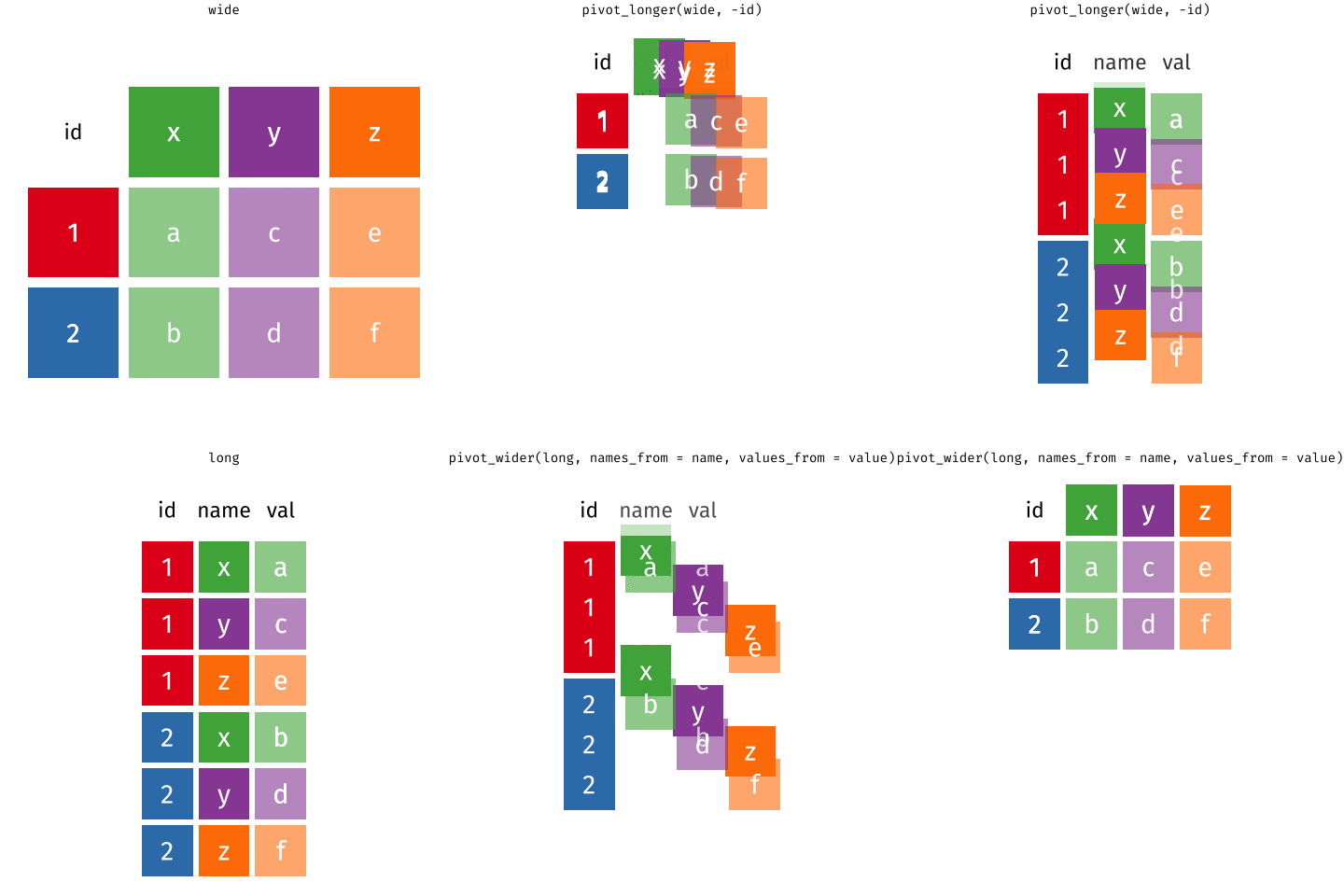
A grammar of data tidying

The goal of tidyr is to help you tidy your data via

pivoting for going between wide and long data
splitting and combining character columns
nesting and unnesting columns
clarifying how NAs should be treated

Pivoting data

Waste characterisation data

objid	location	pet	metal_alu	glass	paper	recyclable	non_recyclable	total
900	eth	0.06	0.06	0.58	0.21	0.92	1.14	2.05
899	eth	0.14	0.01	0.18	0.28	0.61	3.04	3.64
921	old_town	0.00	0.00	0.00	0.41	0.41	1.57	1.99
916	old_town	0.17	0.04	0.80	0.55	1.56	0.62	2.19
900	eth	0.10	0.04	0.00	0.40	0.54	0.58	1.12
899	eth	0.08	0.03	0.00	0.05	0.16	0.34	0.50
921	old_town	0.08	0.03	0.30	0.40	0.81	1.52	2.33
916	old_town	0.11	0.04	0.92	1.01	2.08	1.99	4.07

How would you plot this?

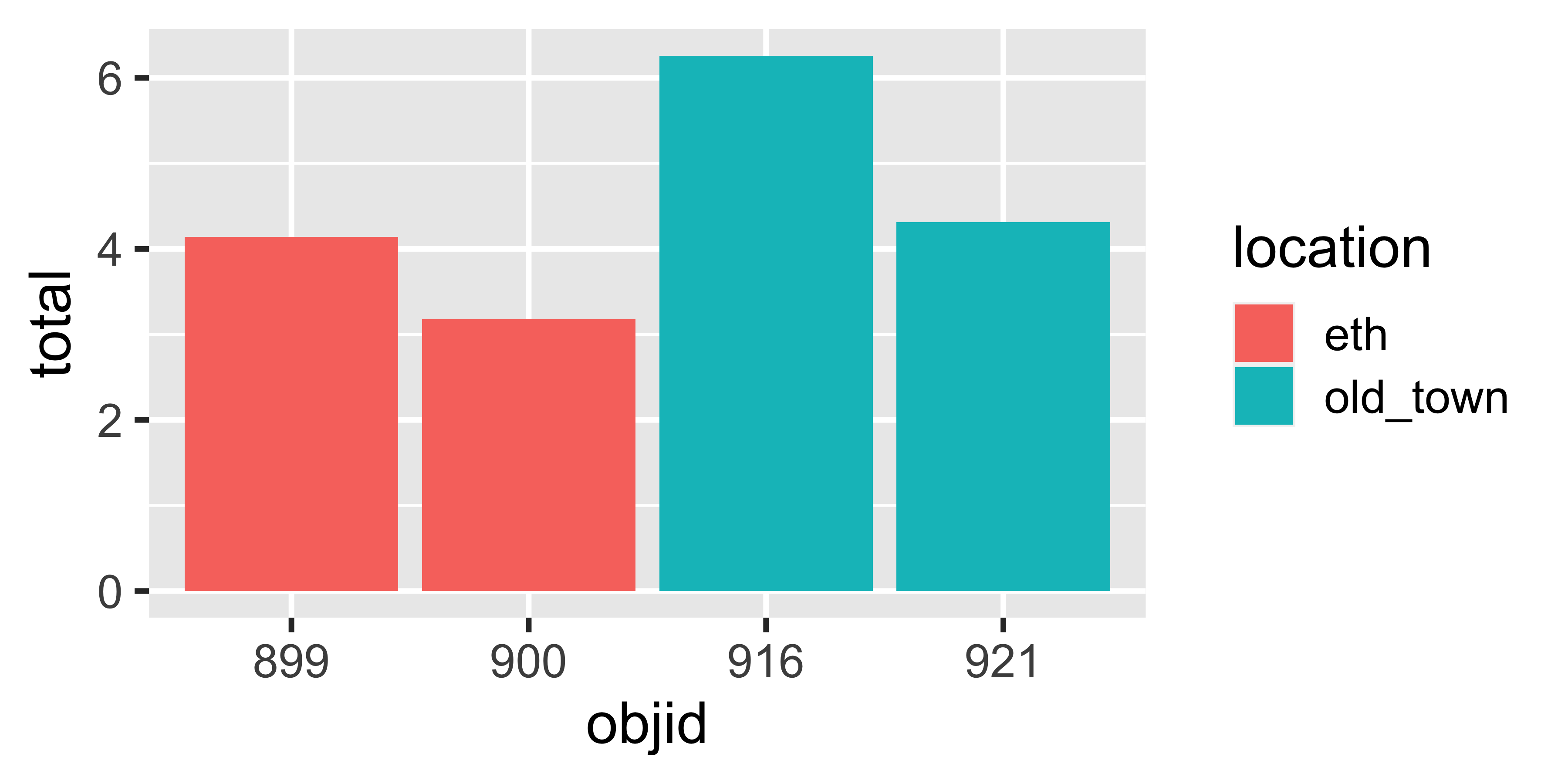
And this?

You need: A long format

objid	location	waste_category	weight
900	eth	pet	0.06
900	eth	metal_alu	0.06
900	eth	glass	0.58
900	eth	paper	0.21
900	eth	other	1.14
899	eth	pet	0.14
899	eth	metal_alu	0.01
899	eth	glass	0.18
899	eth	paper	0.28
899	eth	other	3.04
921	old_town	pet	0.00
921	old_town	metal_alu	0.00
921	old_town	glass	0.00
921	old_town	paper	0.41
921	old_town	other	1.57
916	old_town	pet	0.17
916	old_town	metal_alu	0.04
916	old_town	glass	0.80
916	old_town	paper	0.55
916	old_town	other	0.62
900	eth	pet	0.10
900	eth	metal_alu	0.04
900	eth	glass	0.00
900	eth	paper	0.40
900	eth	other	0.58
899	eth	pet	0.08
899	eth	metal_alu	0.03
899	eth	glass	0.00
899	eth	paper	0.05
899	eth	other	0.34
921	old_town	pet	0.08
921	old_town	metal_alu	0.03
921	old_town	glass	0.30
921	old_town	paper	0.40
921	old_town	other	1.52
916	old_town	pet	0.11
916	old_town	metal_alu	0.04
916	old_town	glass	0.92
916	old_town	paper	1.01
916	old_town	other	1.99

Reminder: The wide format

objid	location	pet	metal_alu	glass	paper	recyclable	non_recyclable	total
900	eth	0.06	0.06	0.58	0.21	0.92	1.14	2.05
899	eth	0.14	0.01	0.18	0.28	0.61	3.04	3.64
921	old_town	0.00	0.00	0.00	0.41	0.41	1.57	1.99
916	old_town	0.17	0.04	0.80	0.55	1.56	0.62	2.19
900	eth	0.10	0.04	0.00	0.40	0.54	0.58	1.12
899	eth	0.08	0.03	0.00	0.05	0.16	0.34	0.50
921	old_town	0.08	0.03	0.30	0.40	0.81	1.52	2.33
916	old_town	0.11	0.04	0.92	1.01	2.08	1.99	4.07

Or this?

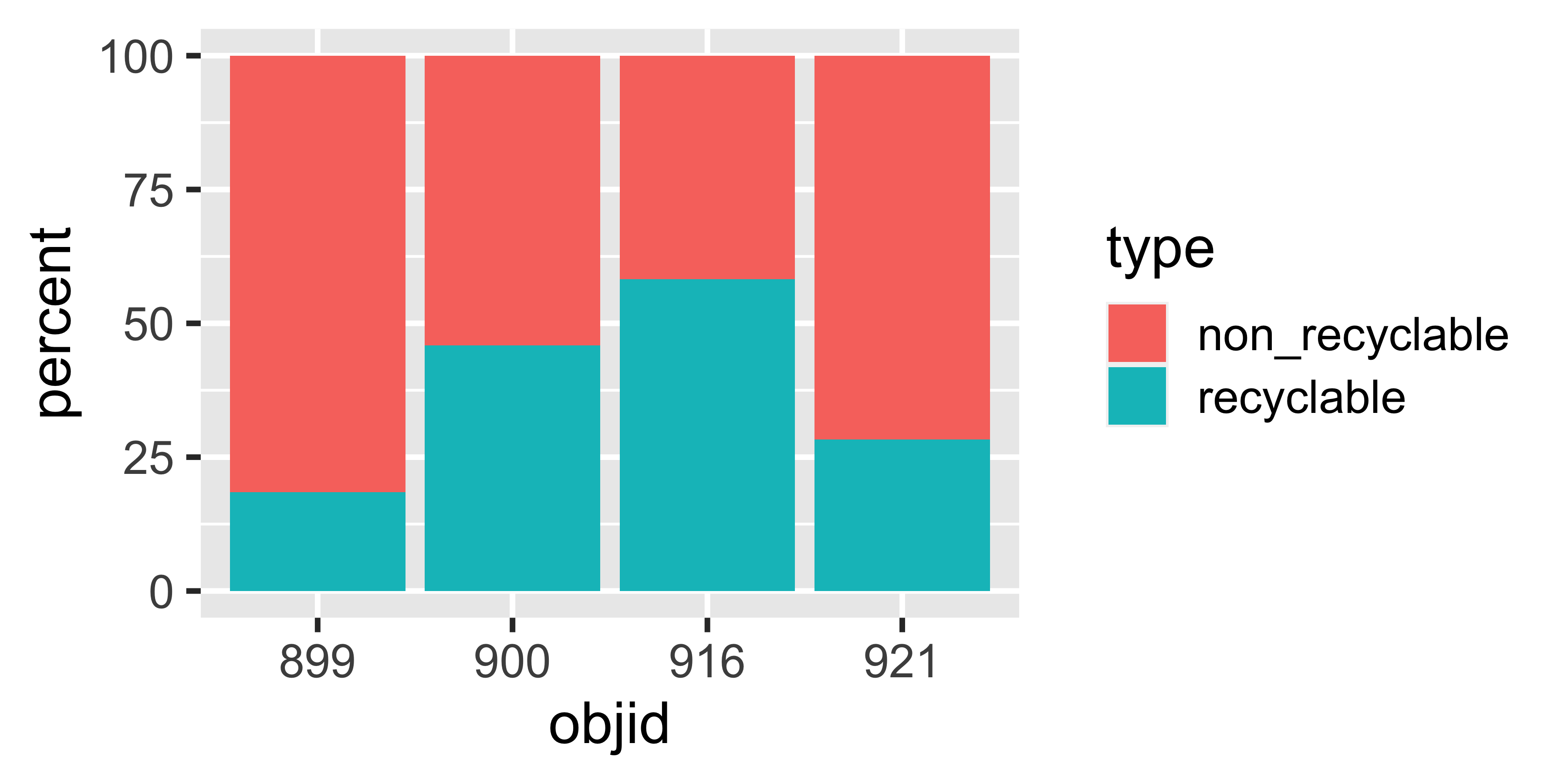
Calculate percentages

objid	location	waste_category	type	weight	percent
900	eth	pet	recyclable	0.06	2.02
900	eth	metal_alu	recyclable	0.06	1.95
900	eth	glass	recyclable	0.58	18.14
900	eth	paper	recyclable	0.21	6.74
900	eth	other	non_recyclable	1.14	35.78
899	eth	pet	recyclable	0.14	3.33
899	eth	metal_alu	recyclable	0.01	0.31
899	eth	glass	recyclable	0.18	4.30
899	eth	paper	recyclable	0.28	6.69
899	eth	other	non_recyclable	3.04	73.36
921	old_town	pet	recyclable	0.00	0.00
921	old_town	metal_alu	recyclable	0.00	0.00
921	old_town	glass	recyclable	0.00	0.00
921	old_town	paper	recyclable	0.41	9.60
921	old_town	other	non_recyclable	1.57	36.46
916	old_town	pet	recyclable	0.17	2.76
916	old_town	metal_alu	recyclable	0.04	0.69
916	old_town	glass	recyclable	0.80	12.73
916	old_town	paper	recyclable	0.55	8.82
916	old_town	other	non_recyclable	0.62	9.99
900	eth	pet	recyclable	0.10	3.09
900	eth	metal_alu	recyclable	0.04	1.35
900	eth	glass	recyclable	0.00	0.00
900	eth	paper	recyclable	0.40	12.60
900	eth	other	non_recyclable	0.58	18.33
899	eth	pet	recyclable	0.08	1.86
899	eth	metal_alu	recyclable	0.03	0.72
899	eth	glass	recyclable	0.00	0.00
899	eth	paper	recyclable	0.05	1.26
899	eth	other	non_recyclable	0.34	8.16
921	old_town	pet	recyclable	0.08	1.81
921	old_town	metal_alu	recyclable	0.03	0.70
921	old_town	glass	recyclable	0.30	6.89
921	old_town	paper	recyclable	0.40	9.32
921	old_town	other	non_recyclable	1.52	35.21
916	old_town	pet	recyclable	0.11	1.74
916	old_town	metal_alu	recyclable	0.04	0.70
916	old_town	glass	recyclable	0.92	14.63
916	old_town	paper	recyclable	1.01	16.20
916	old_town	other	non_recyclable	1.99	31.73

How to

waste_data_untidy

objid	location	pet	metal_alu	glass	paper	recyclable	non_recyclable	total
900	eth	0.06	0.06	0.58	0.21	0.92	1.14	2.05
899	eth	0.14	0.01	0.18	0.28	0.61	3.04	3.64
921	old_town	0.00	0.00	0.00	0.41	0.41	1.57	1.99
916	old_town	0.17	0.04	0.80	0.55	1.56	0.62	2.19
900	eth	0.10	0.04	0.00	0.40	0.54	0.58	1.12
899	eth	0.08	0.03	0.00	0.05	0.16	0.34	0.50
921	old_town	0.08	0.03	0.30	0.40	0.81	1.52	2.33
916	old_town	0.11	0.04	0.92	1.01	2.08	1.99	4.07

How to

waste_data_untidy %>% 
  select(objid:paper, non_recyclable)

objid	location	pet	metal_alu	glass	paper	non_recyclable
900	eth	0.06	0.06	0.58	0.21	1.14
899	eth	0.14	0.01	0.18	0.28	3.04
921	old_town	0.00	0.00	0.00	0.41	1.57
916	old_town	0.17	0.04	0.80	0.55	0.62
900	eth	0.10	0.04	0.00	0.40	0.58
899	eth	0.08	0.03	0.00	0.05	0.34
921	old_town	0.08	0.03	0.30	0.40	1.52
916	old_town	0.11	0.04	0.92	1.01	1.99

How to

waste_data_untidy %>% 
  select(objid:paper, non_recyclable) %>% 
  rename(other = non_recyclable)

objid	location	pet	metal_alu	glass	paper	other
900	eth	0.06	0.06	0.58	0.21	1.14
899	eth	0.14	0.01	0.18	0.28	3.04
921	old_town	0.00	0.00	0.00	0.41	1.57
916	old_town	0.17	0.04	0.80	0.55	0.62
900	eth	0.10	0.04	0.00	0.40	0.58
899	eth	0.08	0.03	0.00	0.05	0.34
921	old_town	0.08	0.03	0.30	0.40	1.52
916	old_town	0.11	0.04	0.92	1.01	1.99

How to

waste_category_levels <- c("glass", "metal_alu", "paper", "pet", "other")

waste_data_untidy %>% 
  select(objid:paper, non_recyclable) %>% 
  rename(other = non_recyclable) %>% 
  pivot_longer(cols = pet:other,
               names_to = "waste_category",
               values_to = "weight") %>% 
  mutate(waste_category = factor(waste_category, 
                                 levels = waste_category_levels))

objid	location	waste_category	weight
900	eth	pet	0.06
900	eth	metal_alu	0.06
900	eth	glass	0.58
900	eth	paper	0.21
900	eth	other	1.14
899	eth	pet	0.14
899	eth	metal_alu	0.01
899	eth	glass	0.18
899	eth	paper	0.28
899	eth	other	3.04
921	old_town	pet	0.00
921	old_town	metal_alu	0.00
921	old_town	glass	0.00
921	old_town	paper	0.41
921	old_town	other	1.57
916	old_town	pet	0.17
916	old_town	metal_alu	0.04
916	old_town	glass	0.80
916	old_town	paper	0.55
916	old_town	other	0.62
900	eth	pet	0.10
900	eth	metal_alu	0.04
900	eth	glass	0.00
900	eth	paper	0.40
900	eth	other	0.58
899	eth	pet	0.08
899	eth	metal_alu	0.03
899	eth	glass	0.00
899	eth	paper	0.05
899	eth	other	0.34
921	old_town	pet	0.08
921	old_town	metal_alu	0.03
921	old_town	glass	0.30
921	old_town	paper	0.40
921	old_town	other	1.52
916	old_town	pet	0.11
916	old_town	metal_alu	0.04
916	old_town	glass	0.92
916	old_town	paper	1.01
916	old_town	other	1.99

How to

waste_category_levels <- c("glass", "metal_alu", "paper", "pet", "other")

waste_data_untidy %>% 
  select(objid:paper, non_recyclable) %>% 
  rename(other = non_recyclable) %>% 
  pivot_longer(cols = pet:other,
               names_to = "waste_category",
               values_to = "weight") %>% 
  mutate(waste_category = factor(waste_category, 
                                 levels = waste_category_levels)) %>%
  mutate(type = case_when(
    waste_category == "other" ~ "non_recyclable",
    TRUE ~ "recyclable")) %>% 
  relocate(type, .before = weight)

objid	location	waste_category	type	weight
900	eth	pet	recyclable	0.06
900	eth	metal_alu	recyclable	0.06
900	eth	glass	recyclable	0.58
900	eth	paper	recyclable	0.21
900	eth	other	non_recyclable	1.14
899	eth	pet	recyclable	0.14
899	eth	metal_alu	recyclable	0.01
899	eth	glass	recyclable	0.18
899	eth	paper	recyclable	0.28
899	eth	other	non_recyclable	3.04
921	old_town	pet	recyclable	0.00
921	old_town	metal_alu	recyclable	0.00
921	old_town	glass	recyclable	0.00
921	old_town	paper	recyclable	0.41
921	old_town	other	non_recyclable	1.57
916	old_town	pet	recyclable	0.17
916	old_town	metal_alu	recyclable	0.04
916	old_town	glass	recyclable	0.80
916	old_town	paper	recyclable	0.55
916	old_town	other	non_recyclable	0.62
900	eth	pet	recyclable	0.10
900	eth	metal_alu	recyclable	0.04
900	eth	glass	recyclable	0.00
900	eth	paper	recyclable	0.40
900	eth	other	non_recyclable	0.58
899	eth	pet	recyclable	0.08
899	eth	metal_alu	recyclable	0.03
899	eth	glass	recyclable	0.00
899	eth	paper	recyclable	0.05
899	eth	other	non_recyclable	0.34
921	old_town	pet	recyclable	0.08
921	old_town	metal_alu	recyclable	0.03
921	old_town	glass	recyclable	0.30
921	old_town	paper	recyclable	0.40
921	old_town	other	non_recyclable	1.52
916	old_town	pet	recyclable	0.11
916	old_town	metal_alu	recyclable	0.04
916	old_town	glass	recyclable	0.92
916	old_town	paper	recyclable	1.01
916	old_town	other	non_recyclable	1.99

How to

waste_category_levels <- c("glass", "metal_alu", "paper", "pet", "other")

waste_data_untidy %>% 
  select(objid:paper, non_recyclable) %>% 
  rename(other = non_recyclable) %>% 
  pivot_longer(cols = pet:other,
               names_to = "waste_category",
               values_to = "weight") %>% 
  mutate(waste_category = factor(waste_category, 
                                 levels = waste_category_levels)) %>% 
  mutate(type = case_when(
    waste_category == "other" ~ "non_recyclable",
    TRUE ~ "recyclable")) %>% 
  relocate(type, .before = weight) %>% 
  group_by(objid) %>% 
  mutate(percent = weight / sum(weight) * 100)

objid	location	waste_category	type	weight	percent
900	eth	pet	recyclable	0.06	2.02
900	eth	metal_alu	recyclable	0.06	1.95
900	eth	glass	recyclable	0.58	18.14
900	eth	paper	recyclable	0.21	6.74
900	eth	other	non_recyclable	1.14	35.78
899	eth	pet	recyclable	0.14	3.33
899	eth	metal_alu	recyclable	0.01	0.31
899	eth	glass	recyclable	0.18	4.30
899	eth	paper	recyclable	0.28	6.69
899	eth	other	non_recyclable	3.04	73.36
921	old_town	pet	recyclable	0.00	0.00
921	old_town	metal_alu	recyclable	0.00	0.00
921	old_town	glass	recyclable	0.00	0.00
921	old_town	paper	recyclable	0.41	9.60
921	old_town	other	non_recyclable	1.57	36.46
916	old_town	pet	recyclable	0.17	2.76
916	old_town	metal_alu	recyclable	0.04	0.69
916	old_town	glass	recyclable	0.80	12.73
916	old_town	paper	recyclable	0.55	8.82
916	old_town	other	non_recyclable	0.62	9.99
900	eth	pet	recyclable	0.10	3.09
900	eth	metal_alu	recyclable	0.04	1.35
900	eth	glass	recyclable	0.00	0.00
900	eth	paper	recyclable	0.40	12.60
900	eth	other	non_recyclable	0.58	18.33
899	eth	pet	recyclable	0.08	1.86
899	eth	metal_alu	recyclable	0.03	0.72
899	eth	glass	recyclable	0.00	0.00
899	eth	paper	recyclable	0.05	1.26
899	eth	other	non_recyclable	0.34	8.16
921	old_town	pet	recyclable	0.08	1.81
921	old_town	metal_alu	recyclable	0.03	0.70
921	old_town	glass	recyclable	0.30	6.89
921	old_town	paper	recyclable	0.40	9.32
921	old_town	other	non_recyclable	1.52	35.21
916	old_town	pet	recyclable	0.11	1.74
916	old_town	metal_alu	recyclable	0.04	0.70
916	old_town	glass	recyclable	0.92	14.63
916	old_town	paper	recyclable	1.01	16.20
916	old_town	other	non_recyclable	1.99	31.73

Live Coding Exercise

ae-13-data-wrangling-tidyr

Back to ae-13a-tidyr.qmd

Break Two

10:00

Part 3: dplyr - joining data

We…

…have multiple data frames

…want to bring them together

professions <- read_csv(here::here("data/scientists/professions.csv"))
dates <- read_csv(here::here("data/scientists/dates.csv"))
works <- read_csv(here::here("scientists/works.csv"))

Data: Women in science

Information on 10 women in science who changed the world

name
Ada Lovelace
Marie Curie
Janaki Ammal
Chien-Shiung Wu
Katherine Johnson
Rosalind Franklin
Vera Rubin
Gladys West
Flossie Wong-Staal
Jennifer Doudna

name	profession
Ada Lovelace	Mathematician
Marie Curie	Physicist and Chemist
Janaki Ammal	Botanist
Chien-Shiung Wu	Physicist
Katherine Johnson	Mathematician
Rosalind Franklin	Chemist
Vera Rubin	Astronomer
Gladys West	Mathematician
Flossie Wong-Staal	Virologist and Molecular Biologist
Jennifer Doudna	Biochemist

name	birth_year	death_year
Janaki Ammal	1897	1984
Chien-Shiung Wu	1912	1997
Katherine Johnson	1918	2020
Rosalind Franklin	1920	1958
Vera Rubin	1928	2016
Gladys West	1930	NA
Flossie Wong-Staal	1947	NA
Jennifer Doudna	1964	NA

name	known_for
Ada Lovelace	first computer algorithm
Marie Curie	theory of radioactivity, discovery of elements polonium and radium, first woman to win a Nobel Prize
Janaki Ammal	hybrid species, biodiversity protection
Chien-Shiung Wu	confim and refine theory of radioactive beta decy, Wu experiment overturning theory of parity
Katherine Johnson	calculations of orbital mechanics critical to sending the first Americans into space
Vera Rubin	existence of dark matter
Gladys West	mathematical modeling of the shape of the Earth which served as the foundation of GPS technology
Flossie Wong-Staal	first scientist to clone HIV and create a map of its genes which led to a test for the virus
Jennifer Doudna	one of the primary developers of CRISPR, a ground-breaking technology for editing genomes

Desired output

name	profession	birth_year	death_year	known_for
Ada Lovelace	Mathematician	NA	NA	first computer algorithm
Marie Curie	Physicist and Chemist	NA	NA	theory of radioactivity, discovery of elements polonium and radium, first woman to win a Nobel Prize
Janaki Ammal	Botanist	1897	1984	hybrid species, biodiversity protection
Chien-Shiung Wu	Physicist	1912	1997	confim and refine theory of radioactive beta decy, Wu experiment overturning theory of parity
Katherine Johnson	Mathematician	1918	2020	calculations of orbital mechanics critical to sending the first Americans into space
Rosalind Franklin	Chemist	1920	1958	NA
Vera Rubin	Astronomer	1928	2016	existence of dark matter
Gladys West	Mathematician	1930	NA	mathematical modeling of the shape of the Earth which served as the foundation of GPS technology
Flossie Wong-Staal	Virologist and Molecular Biologist	1947	NA	first scientist to clone HIV and create a map of its genes which led to a test for the virus
Jennifer Doudna	Biochemist	1964	NA	one of the primary developers of CRISPR, a ground-breaking technology for editing genomes

Inputs, reminder

names(professions)

[1] "name"       "profession"

names(dates)

[1] "name"       "birth_year" "death_year"

names(works)

[1] "name"      "known_for"

nrow(professions)

[1] 10

nrow(dates)

[1] 8

nrow(works)

[1] 9

Joining data frames

something_join(x, y)

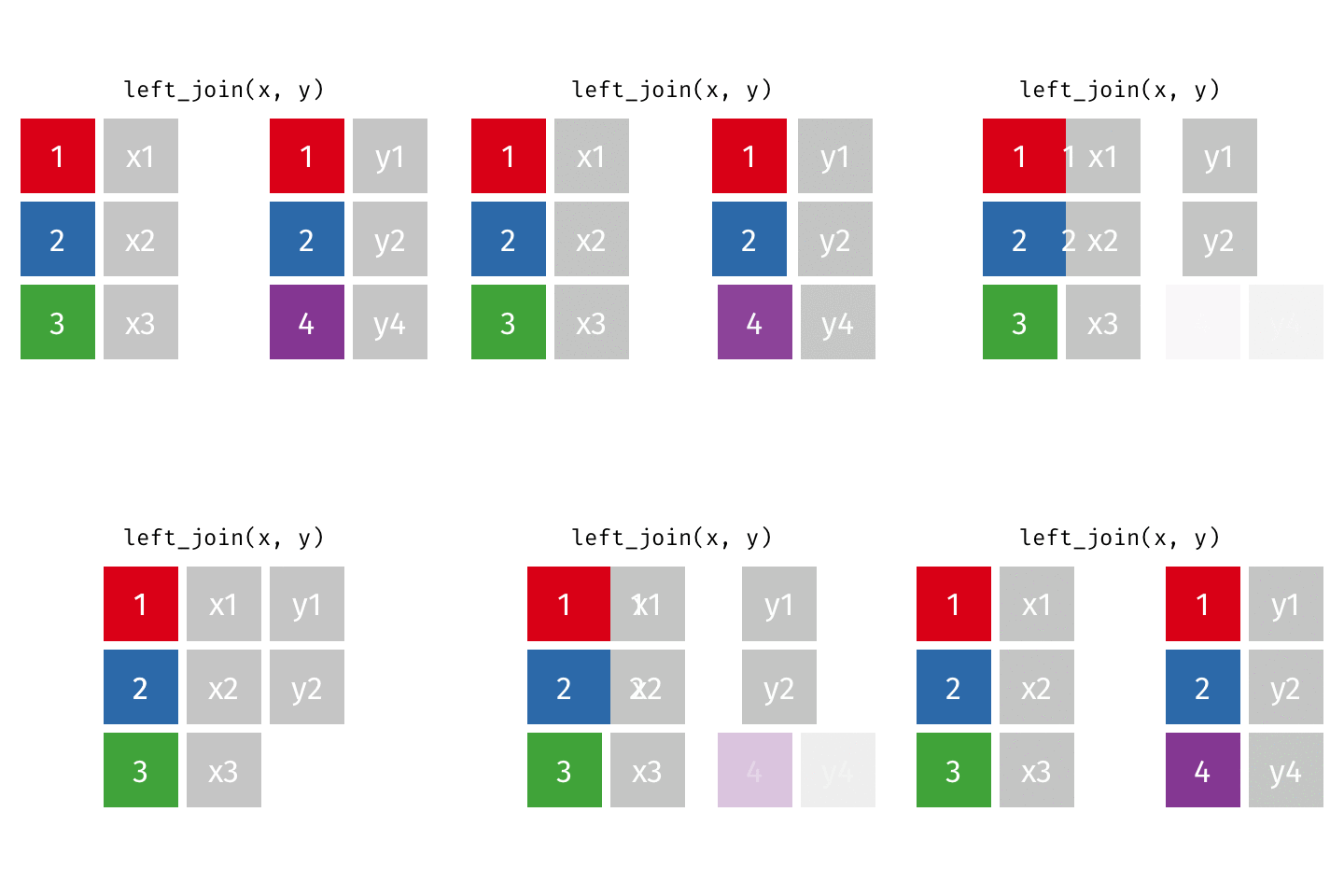
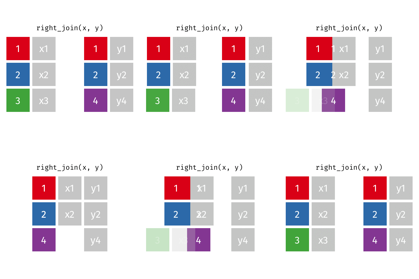
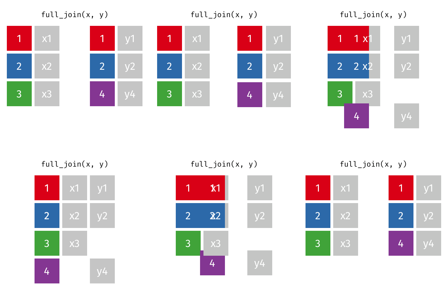
left_join(): all rows from x
right_join(): all rows from y
full_join(): all rows from both x and y
…

Setup

For the next few slides…

x <- tibble(
  id = c(1, 2, 3),
  value_x = c("x1", "x2", "x3")
  )

# A tibble: 3 × 2
     id value_x
  <dbl> <chr>  
1     1 x1     
2     2 x2     
3     3 x3

y <- tibble(
  id = c(1, 2, 4),
  value_y = c("y1", "y2", "y4")
  )

# A tibble: 3 × 2
     id value_y
  <dbl> <chr>  
1     1 y1     
2     2 y2     
3     4 y4

`left_join()`

left_join(x, y)

# A tibble: 3 × 3
     id value_x value_y
  <dbl> <chr>   <chr>  
1     1 x1      y1     
2     2 x2      y2     
3     3 x3      <NA>

`left_join()`

professions %>%
  left_join(dates)

# A tibble: 10 × 4
  name              profession            birth_year death_year
  <chr>             <chr>                      <dbl>      <dbl>
1 Ada Lovelace      Mathematician                 NA         NA
2 Marie Curie       Physicist and Chemist         NA         NA
3 Janaki Ammal      Botanist                    1897       1984
4 Chien-Shiung Wu   Physicist                   1912       1997
5 Katherine Johnson Mathematician               1918       2020
6 Rosalind Franklin Chemist                     1920       1958
# … with 4 more rows

`right_join()`

right_join(x, y)

# A tibble: 3 × 3
     id value_x value_y
  <dbl> <chr>   <chr>  
1     1 x1      y1     
2     2 x2      y2     
3     4 <NA>    y4

`right_join()`

professions %>%
  right_join(dates)

# A tibble: 8 × 4
  name              profession    birth_year death_year
  <chr>             <chr>              <dbl>      <dbl>
1 Janaki Ammal      Botanist            1897       1984
2 Chien-Shiung Wu   Physicist           1912       1997
3 Katherine Johnson Mathematician       1918       2020
4 Rosalind Franklin Chemist             1920       1958
5 Vera Rubin        Astronomer          1928       2016
6 Gladys West       Mathematician       1930         NA
# … with 2 more rows

`full_join()`

full_join(x, y)

# A tibble: 4 × 3
     id value_x value_y
  <dbl> <chr>   <chr>  
1     1 x1      y1     
2     2 x2      y2     
3     3 x3      <NA>   
4     4 <NA>    y4

`full_join()`

dates %>%
  full_join(works)

# A tibble: 10 × 4
  name              birth_year death_year known_for              
  <chr>                  <dbl>      <dbl> <chr>                  
1 Janaki Ammal            1897       1984 hybrid species, biodiv…
2 Chien-Shiung Wu         1912       1997 confim and refine theo…
3 Katherine Johnson       1918       2020 calculations of orbita…
4 Rosalind Franklin       1920       1958 <NA>                   
5 Vera Rubin              1928       2016 existence of dark matt…
6 Gladys West             1930         NA mathematical modeling …
# … with 4 more rows

Putting it altogether

professions %>%
  left_join(dates) %>%
  left_join(works)

# A tibble: 10 × 5
  name              profession    birth_year death_year known_for
  <chr>             <chr>              <dbl>      <dbl> <chr>    
1 Ada Lovelace      Mathematician         NA         NA first co…
2 Marie Curie       Physicist an…         NA         NA theory o…
3 Janaki Ammal      Botanist            1897       1984 hybrid s…
4 Chien-Shiung Wu   Physicist           1912       1997 confim a…
5 Katherine Johnson Mathematician       1918       2020 calculat…
6 Rosalind Franklin Chemist             1920       1958 <NA>     
# … with 4 more rows

Live Coding Exercise

ae-13-data-wrangling-tidyr

Back to ae-13a-tidyr.qmd

Homework Assignment

Submission

All details in assignment week 13
Due: Wednesday, 26th May at 23:59 (2 points)

Evaluation

5 mins
anonymous
after each lecture

kutt.it/rbtl-eval

Programming

ae-13-data-wrangling-tidyr

Open the file: ae-13b-dplyr.qmd
Work through the exercises
Finalise as part of your homework

Thanks! 🌻

A large proportion of slides in this presentation are either taken from or adapted from Data Science in a Box]

Slides created via revealjs and Quarto: https://quarto.org/docs/presentations/revealjs/ Access slides as PDF on GitHub

All material is licensed under Creative Commons Attribution Share Alike 4.0 International.